This post contains the notes taken from reading of the following paper:
I was also helped by the slides of Stanford’s CS231b.
Fast-RCNN was the state-of-the-art algorithm for object detection in 2015; its object proposal used Selective Search that itself used Efficient Graph-Based Segmentation.
The reason this segmentation was still useful almost 10 years later is because the algorithm is fast, while remaining efficient. Its goal is to segment the objects in an image.
A Graph-Based Algorithm
The algorithm sees an image as a graph, and every pixels as vertices. Making of good segmentation for an image is thus equivalent to finding communities in a graph.
What separates two communities of pixels is a boundary based on where similarity ends and dissimilarity begins. A segmentation too fine would result in communities separated without real boundary between them; in a segmentation too coarse communities should be splitted.

The authors of the papers argue that their algorithm always find the right segmentation, neither too fine nor too coarse.
Predicate Of A Boundary
The authors define their algorithm with a predicate $D$ that measures dissimilarity: That predicate takes two components and returns true if a boundary exists between them. A component is a segmentation of one or more vertice.
With $C1$ and $C2$ two components:
$$ D(C1, C2) = \begin{cases} true & \text{if } \text{Dif}(C1, C2) > \text{MInt}(C1, C2)\newline false & \text{otherwise} \end{cases} $$
With:
$$\text{Dif}(C1, C2) = \min_{\substack{v_i \in C1, v_j \in C2 \newline (v_i, v_j) \in E_{ij}}} w(v_i, v_j)$$
The function $Dif(C1, C2)$ returns the minimum weight $w(.)$ edge that connects a vertice $v_i$ to $v_j$, each of them being in two different components. $E_{ij}$ is the set of edges connecting two vertices between components $C1$ and $C2$. This function $Dif$ measures the difference between two components.
And with:
$$\text{MInt}(C1, C2) = min (\text{Int}(C1) + \tau(C1), \text{Int}(C2) + \tau(C2))$$
$$\tau(C) = \frac{k}{|C|}$$
$$\text{Int}(C) = \max_{\substack{e \in \text{MST}(C, E)}} w(e)$$
The function $\text{Int}(C)$ returns the edge with maximum weight that connects two vertices in the Minimum Spanning Tree (MST) of a same component. Looking only in the MST reduces considerably the number of possible edges to consider: A spanning tree has $n - 1$ edges instead of the $\frac{n(n - 1)}{2}$ total edges. Moreover, using the minimum spanning tree and not just a common spanning tree allows to have segmentation with high-variability (but still progressive). This function $\text{Int}$ measures the internal difference of a component. A low $\text{Int}$ means that the component is homogeneous.
The function $\tau(C)$ is a threshold function, that imposes a stronger evidence of boundary for small components. A large $k$ creates a segmentation with large components. The authors set $k = 300$ for wide images, and $k = 150$ for detailed images.
Finally $\text{MInt}(C1, C2)$ is the minimum of internal difference of two components.
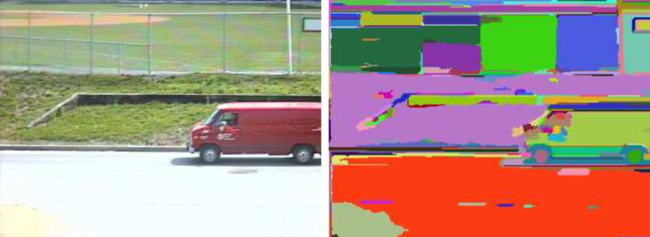
To summarize the predicate $D$: A large difference between two internally homogeneous components is evidence of a boundary between them. However, if the two components are internally heterogeneous it would be harder to prove a boundary. Therefore details are ignored in high-variability regions but are preserved in low-variability regions:

Notice how the highly-variable grass is correctly segmented while details like numbers on the back of the first player are preserved.
Different Weight Functions
The predicate uses a function $w(v_i, v_j)$ that measures the edge’s weight between two vertices $v_i$ and $v_j$.
The authors provide two alternatives for this weight function:
Grid Graph Weight
To correctly use this weight function, the authors smooth the image using a Gaussian filter with $\sigma = 0.8$.
The Grid Graph Weight function is:
$$w(v_j, v_i) = |I(p_i) - I(p_j)|$$
It is the intensity’s difference of the pixel neighbourhood. Indeed, the authors choose to not only use the pixel intensity, but also its 8 neighbours.
 The intensity is the pixel-value of the central pixel $p_i$ and its 8
neighbours.
The intensity is the pixel-value of the central pixel $p_i$ and its 8
neighbours.
Using this weight function, they run the algorithm three times (for red, blue, and green) and choose the intersection of the three segmentations as result.
Nearest Neighbours Graph Weight
The second weight function is based on the Approximate Nearest Neighbours Search.
It tries to find a good approximation of what could be the closest pixel. The features space is both the spatial coordinates and the pixel’s RGB.
Features Space = $(x, y, r, g, b)$.
The Actual Algorithm
Now that every sub-function of the algorithm has been defined, let’s see the actual algorithm:
For the Graph $G = (V, E)$ composed of the vertices $V$ and the edges $E$, and a segmentation $S = (C_1, C_2, …)$:
- Sort E into $\pi$ = ($o_1$, …, $o_m$) by increasing edge weight order.
- Each vertice is alone in its own component. This is the initial segmentation $S^0$.
- For $q = 1, …, m$:
- Current segmentation is $S^q$
- ($v_i$, $v_j$) $= o_q$
- If $v_i$ and $v_j$ are not in the same component, and the predicate
$D(C_i^{q - 1}, C_j^{q - 1})$ is false then:
- Merge $C_i$ and $C_j$ into a single component.
- Return $S^m$.
The superscript $q$ in $S^q$ or $C_x^Q$ simply denotes a version of the segmentation or of the component at the instant $q$ of the algorithm.
Basically what the algorithm is doing is a bottom-up merging of at first individual pixels into larger and larger components. At the end, the segmentation $S^m$ will neither be too fine nor too coarse.

Conclusion
As you have seen, the algorithm of this paper is quite simple. What makes it efficient is the chosen metrics and the predicate defined beforehand.
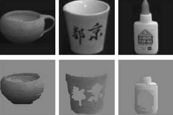
If you have read until the bottom of the page, congrats! To thank you, here is some demonstrations by the authors: