The hallmark of human intelligence is the capacity to learn. A toddler has comparable aptitudes to reason about space, quantities, or causality than other ape species (source). The difference of our cousins and us is the ability to learn from others.
The recent deep learning hype aims to reach the Artificial General Intelligence (AGI): an AI that would express (supra-)human-like intelligence. Unfortunately current deep learning models are flawed in many ways: one of them is that they are unable to learn continuously as human does through years of schooling, and so on.
Why do we want our models to learn continuously?
Regardless of the far away goal of AGI, there are several practicals reasons why we want our model to learn continuously. Before describing a few of them, I’ll mention two constraints:
- Our model cannot review all previous knowledge each time it needs to learn new facts. As a child in 9th grade, you don’t review all the syllabus of 8th grade as it’s supposed to have been already memorized.
- Our model needs to learn continuously without forgetting any previously learned knowledge.
A real applications of these two constraints is robotics: a robot in the wild should learn continuously its environment. Furthermore due to hardware limitation, it may neither store all previous data nor spend too much computational resource.
Another application is what I do at Heuritech: we detect fashion trends. However every day across the globe a new trend may appear. It is impracticable to review our large trends database each time we need to learn a new one.
Now that the necessity of learning continuously has been explained, let us differentiate three scenarios (Lomonaco and Maltoni, 2017):
- Learning new data of known classes (online learning)
- Learning new classes (class-incremental learning)
- The union of the two previous scenarios
In this article I will focus only on the second scenario. Note however that the methods used are fairly similar between scenario.
More practically this article will cover models that learn incrementally new classes. The model will see only new classes’ data, as we aim to remember well old classes. After each task, the model is trained on a all seen classes using a separate test set:
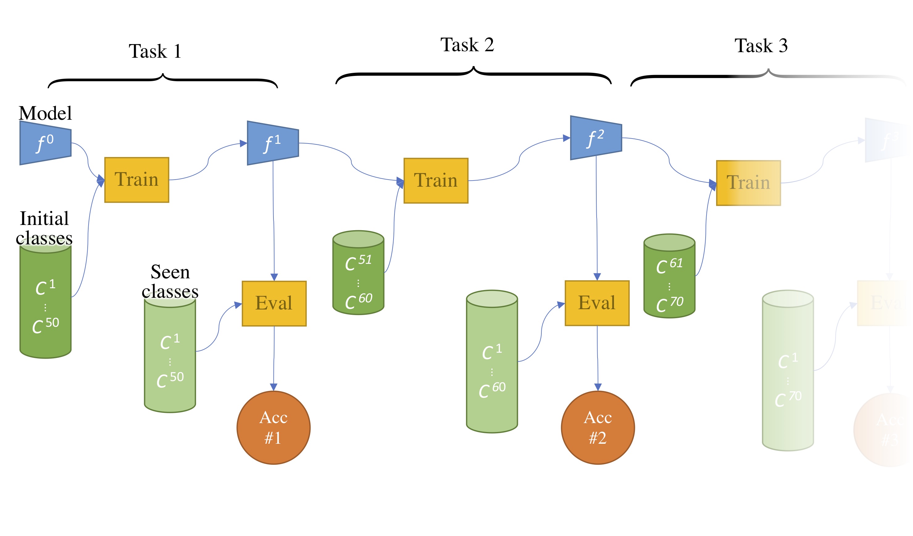
Figure 1: Several steps of incremental learning.
As seen in the image above, each step produces a new accuracy score. Following (Rebuffi et al, 2017) the final score is the average of all previous task accuracy score. It’s called the average incremental accuracy.
Naive solution: transfer learning
Transfer learning allows to transfer the knowledge gained on one task (e.g ImageNet and its 1000 classes) to another task (e.g classify cats & dogs) (Razavian et al, 2014). Usually the backbone (a ConvNet in Computer Vision, like ResNet) is kept while a new classifier is plugged in on top of it. During transfer, we train the new classifier & fine-tune the backbone.
Finetuning the backbone is essential to reach good performance on the destination task. However we don’t have access anymore to the original task data. Therefore our model is now optimized only for the new task. While at the training end, we will have good performance on this new task, the old task will suffer a significant drop of performance.
(French, 1995) described this phenomenon as a catastrophic forgetting. To solve it, we must find an optimal trade-off between rigidity (being good on old tasks) and plasticity (being good on new tasks).
Three broad strategies
(Parisi et al, 2018) defines 3 broad strategies:
- External Memory storing a small amount of previous tasks data
- Constraints-based methods avoiding forgetting on previous tasks
- Model Plasticity extending the capacity
1. External Memory
As said previously we cannot keep all our previous data for several reasons. We can however relax this constraint by limiting access to previous data to a bounded amount.
Rehearsal learning (Rebuffi et al, 2017)’s iCaRL assumes we dispose of a limited amount of space to store previous data. Our external memory could have a capacity of 2,000 images. After learning new classes, a few amount of those classes data could be kept in it while the rest would be discarded.
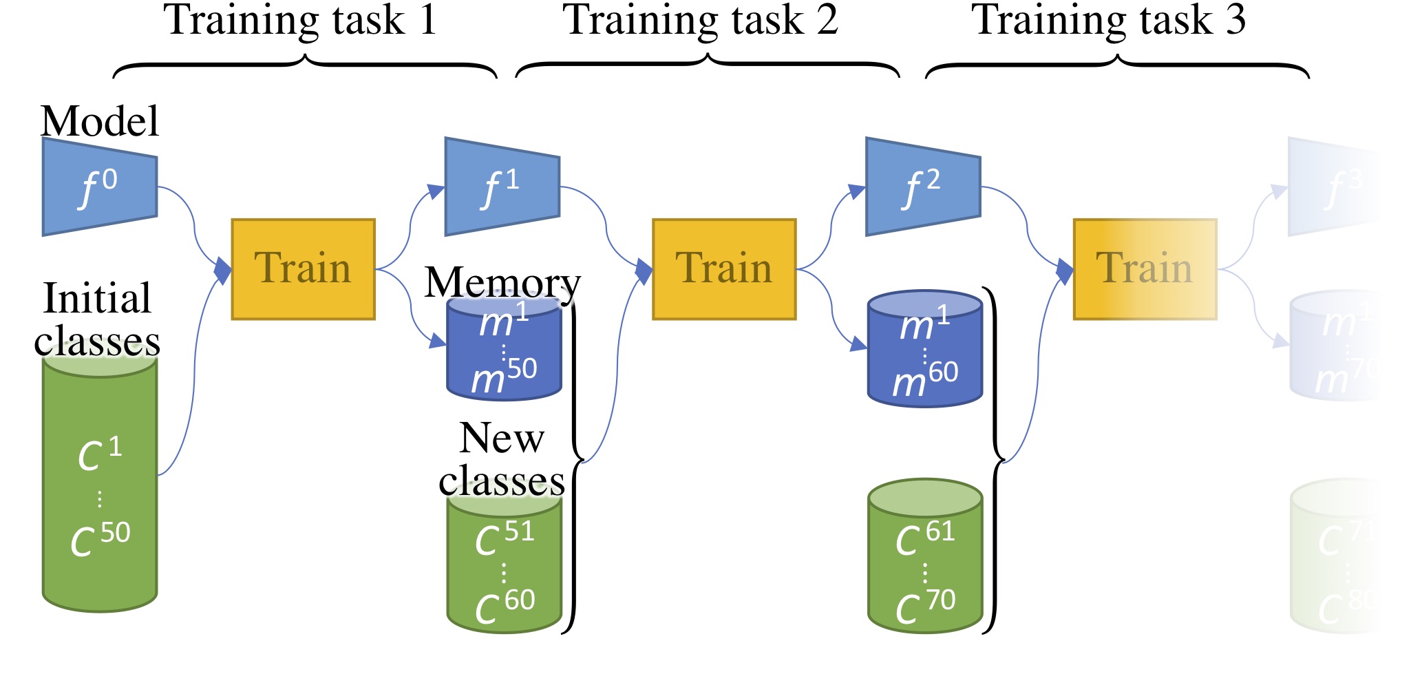
Figure 2: Several steps of incremental learning with a memory storing a subset of previous data.
Pseudo-Rehearsal learning (Shin et al, 2017; Kemker and Kanan, 2018) assume instead that we cannot keep previous data, like images, but that we can store the class distribution statistics. With this, a generative model can generate on-the-fly old classes data. This approach is however very reliant on the quality of the generative model; generated data are still subpar to real data (Ravuri and Vinyals, 2019). Furthermore it is still crucial to also avoid a forgetting in the generator.
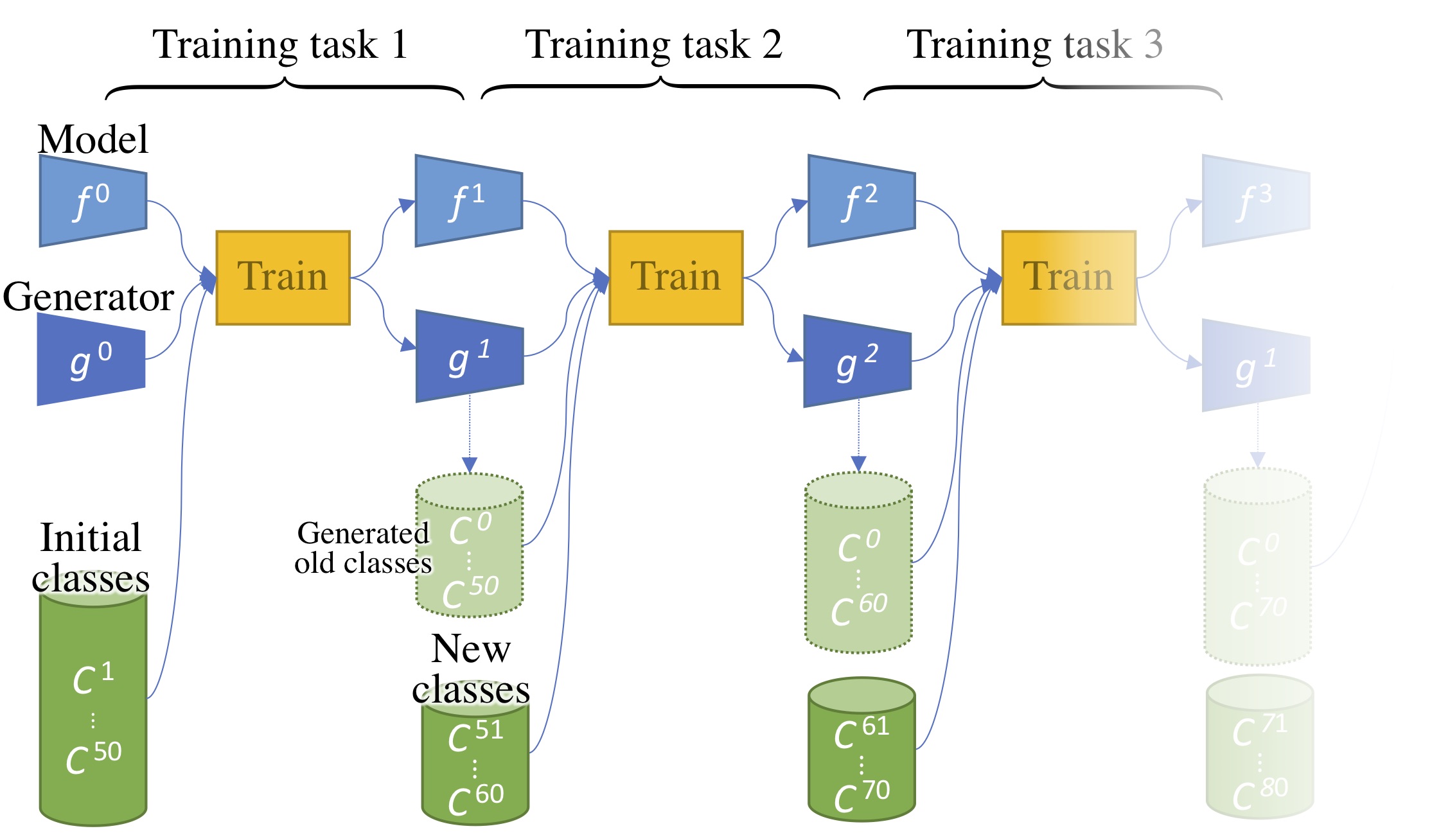
Figure 3: Several steps of incremental learning with a generator generating previous data.
Generally (pseudo-)rehearsal-based methods outperforms methods only using new classes data. It’s then fair to compare their performance separately.
2. Constraints-based methods
Intuitively, forcing the current model $M^t$ to be similar to its previous version $M^{t-1}$ will avoid forgetting. There is a large array of methods aiming to do so. However they all have to balance a rigidity (encouraging similarity between $M^t$ and $M^{t-1}$) and plasticity (letting enough slack to $M^t$ to learn new classes).
We can separate those methods in three broads categories:
- Those enforcing a similarity of the activations
- Those enforcing a similarity of the weights
- And those enforcing a similarity of the gradients
2.1. Constraining the activations
(Li and Hoiem, 2016)’s LwF introduced knowledge distillation from (Hinton et al, 2015): given a same image, $f^t$’s base probabilities should be similar to $f^{t-1}$’s probabilities:
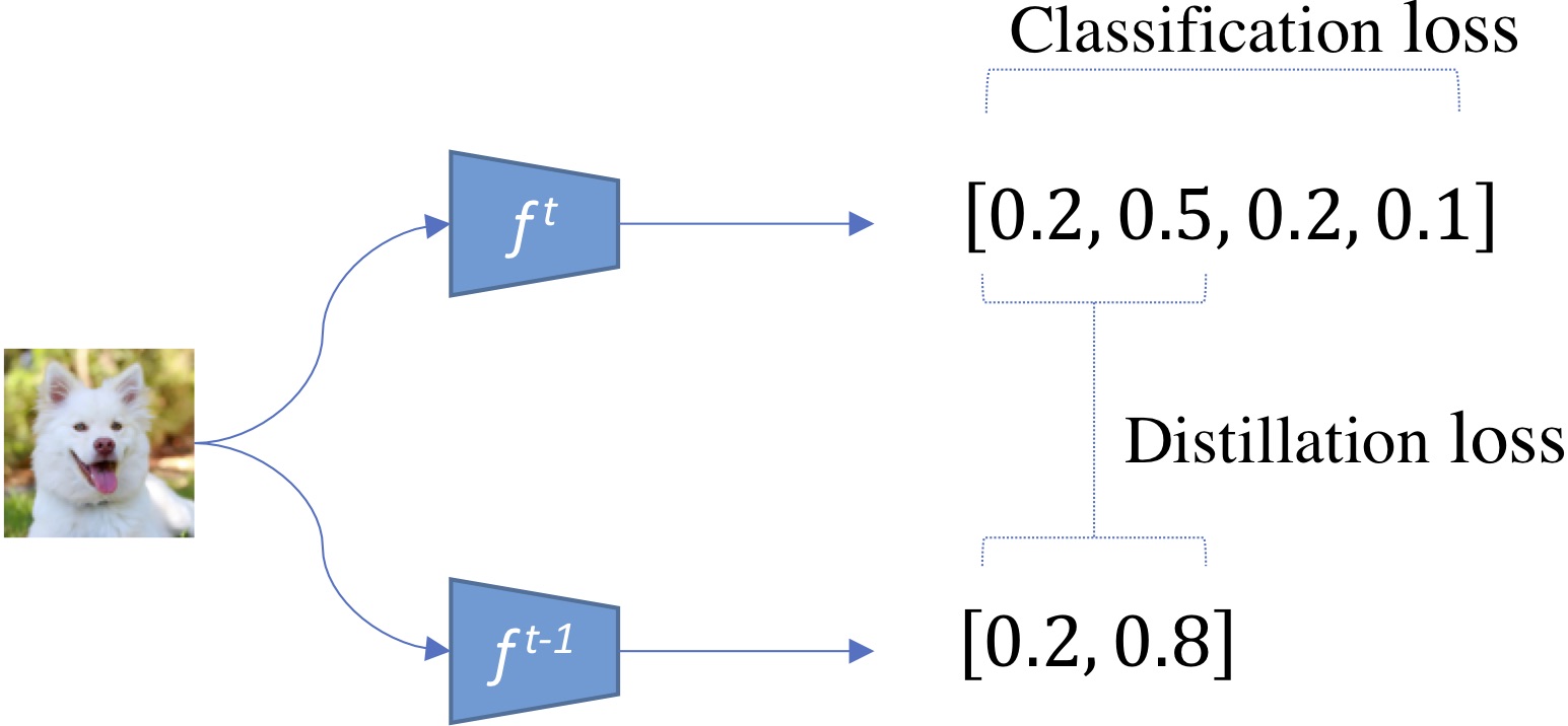
Figure 4: Base probabilities are distilled from the previous model to the new one.
The distillation loss can simply be a binary cross-entropy between old and new probabilities.
Model output probabilities is just one kind of activation among others. (Hou et al, 2019)’s UCIR used a similarity-based between the extracted features $h^{t-1}$ and $h^t$ of the old and new model:
$$L_\text{Less-Forget} = 1-\langle \frac{h^t}{\Vert h^t \Vert_2}, \frac{h^{t-1}}{\Vert h^{t-1} \Vert_2}\rangle$$
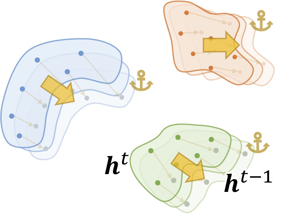
Figure 5: New model embeddings must be similar from the old one.
To sum up, encouraging the new model to mimic the activations of its previous version reduces the forgetting of old classes. A different but similar approach is reduce the difference between the new and old model weights:
2.2. Constraining the weights
A naive method would be to minimize a distance between the new and old weights likewise $L = (\mathbf{W}^t - \mathbf{W}^{t-1})^2$. However, as remarked by (Kirkpatrick et al, 2016)’s EWC, the resulting new weights would be under-performing for both old and new classes. Then, the authors suggested to modulate the regularization according to neurons importance.
Important neurons for task $T-1$ must not change in the new model. On the other hand, unimportant neurons can be more freely modified, to learn efficiently the new task $T$:
$$L = I (W^{t-1} - W^t)^2$$
With $W^{t-1}$ and $W^{t}$ the weights of respectively the old and new model, and $I$ a neurons importance matrix defined from $W^{t-1}$.
In EWC, the neurons importance are defined with the Fisher information, but variants exist. Following research (Zenke et al, 2017; Chaudhry et al, 2018) builds on the same idea with refinement of the neurons importance definition.
2.3. Constraining the gradients
Finally a third category of constraints exist: constraining the gradients. Introduced by (Lopez-Paz and Ranzato, 2017)’s GEM, the key idea is that the the new model’s loss should be lower or equal to the old model’s loss on old samples stored in a memory (cf rehearsal learning).
$$L(f^t, M) \le L(f^{t-1}, M)$$
The authors rephrase this constraint as an angle constraint on the gradients:
$$\langle \frac{\partial L(f^t, M)}{\partial f^t}, \frac{\partial L(f^{t-1}, M)}{\partial f^{t-1}} \rangle \ge 0$$
Put it more simply, we want the gradients of the new model to “go in the same direction” as they would have with the previous model.
If this constraint is respected, it’s likely that the new model won’t forget old classes. Otherwise the incoming gradients $g$ must be “fixed“: they are reprojected to their closest valid alternative $\tilde{g}$ by minimizing this quadratic program:
$$\text{minimize}_{\tilde{g}}\, \Vert g^t - \tilde{g} \Vert_2^2$$
$$\text{subject to}\, \langle g^{t-1}, \tilde{g} \rangle \ge 0$$
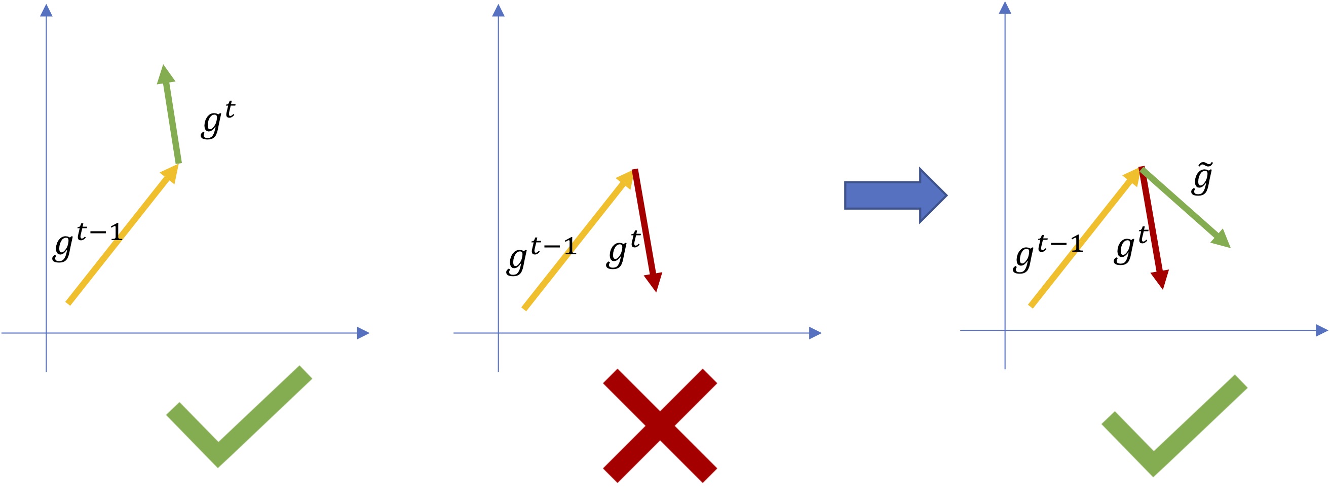
Figure 6: Gradients must keep going in the same direction, otherwise their direction is fixed.
As you may guess, solving this program for each violating gradients, before updating the model weights is very costly in time. (Chaudhry et al, 2018 ; Aljundi et al, 2019) improve the algorithm speed by different manners, including sampling a representative subset of the gradients constraints.
3. Plasticity
Other algorithms modify the network structure to reduce catastrophic forgetting. The first strategy is to add new neurons to the current model. (Yoon et al, 2017)’s DEN first trains on the new task. If its loss is not good enough, new neurons are added at several layers and they will be dedicated to learn on the new task. Furthermore the authors choose to freeze some of the already-existing neurons. Those neurons, that are particularly important for the old tasks, must not change in order to reduce forgetting.
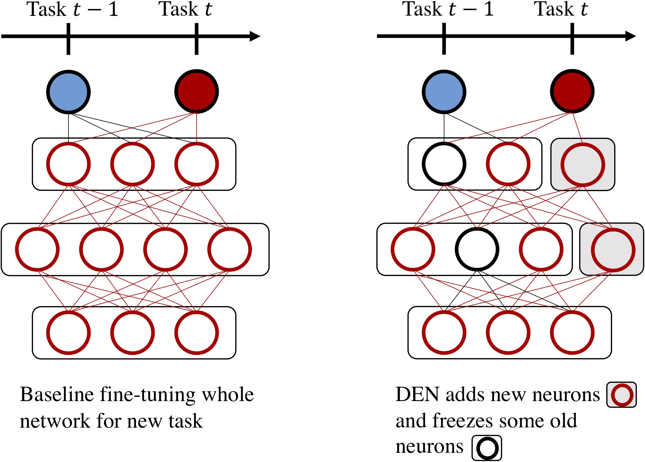
Figure 7: DEN adds new neurons for the new tasks, and selectively fine-tunes existing neurons.
While expanding the network capacity makes sense in an incremental setting where our model learns indefinitely, it’s worth noting that existing deep learning models are over-parametrized. The initial capacity can be enough to learn many tasks, at the condition that it’s used appropriately. As (Frankle and Carbin, 2019)’s Lottery Ticket Hypothesis formalized, large networks are made of very efficient sub-networks.
Each sub-network can be dedicated to only one task:
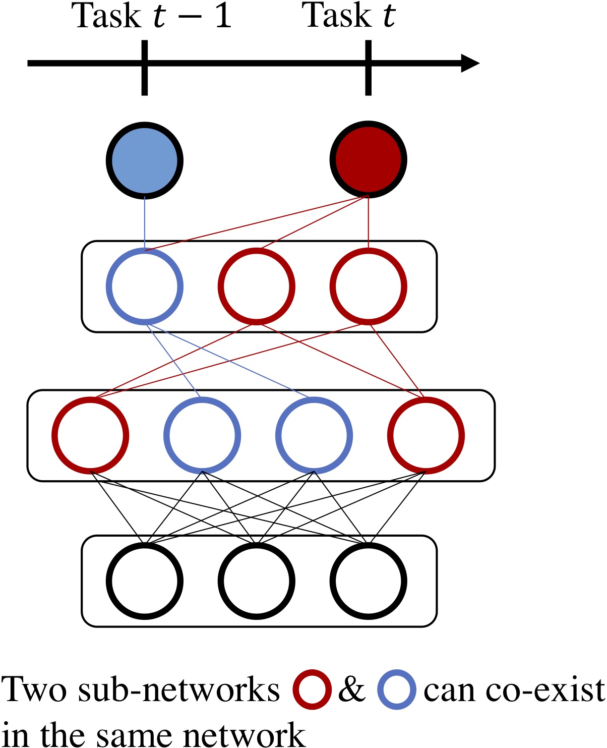
Figure 8: Among a large single network, several subnetworks can be uncovered, each specialized for a task.
Several methods exist to uncover those sub-networks: (Fernando et al, 2017)’s PathNet uses evolutionary algorithm, (Golkar et al, 2019) sparsify the whole network with a L1 regularization, and (Hung et al, 2019)’s CPG learns binary masks activating and deactivating connections to produce sub-networks.
It is worth noting that methods based on sub-networks assume to know on which task they are evaluated on. This setting, called multi-heads is challenging but fundamentally easier than single-head evaluation where models are evaluated on all tasks in the same time.
Dealing with class imbalance
We saw previously three strategy to avoid forgetting (rehearsal, constraints, and plasticity). Those methods can be used together. Rehearsal is often used in addition of constraints.
Moreover another challenge of incremental learning is the large class imbalance between new and old classes. For example, on some benchmarks, new classes could be made of 500 images each, while old classes would only have 20 images each stored in memory.
This class imbalance further encourages, wrongly, the model to be over-confident for new classes while being under-confident for old classes. Catastrophic forgetting is furthermore exacerbated.
(Castro et al, 2018) train for each task their model under this class imbalance, but fine-tune it after with under-sampling: old & new classes are sampled to have as much images.
(Wu et al, 2019) consider to use re-calibration (Guo et al, 2017): a small linear model is learned on validation to “fix” the over-confidence on new classes. It is only applied for new classes logits. (Belouadah and Popescu, 2019) proposed concurrently a similar solution fixing the new classes logits, but using instead class statistics.
(Hou et al, 2019) remarked that weights & biases of the classifier layer have larger magnitude for new classes than older classes. To reduce this effect, they replace the usual classifier by a cosine classifier where weights and features are L2 normalized. Moreover they freeze the classifier weights associated to old classes.
Conclusion
In this article we saw what is incremental learning: learning model with classes coming incrementally; what is its challenge: avoiding forgetting the previous classes to the benefice only of new classes; and broad strategies to solve this domain.
This domain is far from being solved. The upper bound is a model trained in a single step on all data. Current solutions are considerably worse than this.
On a personal note, my team and I have submitted an article for a conference on this subject. If it’s accepted, I’ll make a blog article on it. Furthermore I have made a library to train incremental model: inclearn.