Deep Neural Networks (DNNs) are notorious for requiring less feature engineering than Machine Learning algorithms. For example convolutional networks learn by themselves the right convolution kernels to apply on an image. No need of carefully handcrafted kernels.
However a common point to all kinds of neural networks is the need of normalization. Normalizing is often done on the input, but it can also take place inside the network. In this article I’ll try to describe what the literature is saying about this.
This article is not exhaustive but it tries to cover the major algorithms. If you feel I missed something important, tell me!
Normalizing the input
It is extremely common to normalize the input (lecun-98b), especially for computer vision tasks. Three normalization schemes are often seen:
- Normalizing the pixel values between 0 and 1 (as Torch’s ToTensor does):
img /= 255.- Normalizing the pixel values between -1 and 1 (as Tensorflow does):
img /= 127.5
img -= 1.
Why is it recommended? Let’s take a neuron, where:
$$y = w \cdot x$$
The partial derivative of $y$ for $w$ that we use during backpropagation is:
$$\frac{\partial y}{\partial w} = X^T$$
The scale of the data has an effect on the magnitude of the gradient for the weights. If the gradient is big, you should reduce the learning rate. However you usually have different gradient magnitudes in a same batch. Normalizing the image to smaller pixel values is a cheap price to pay while making easier to tune an optimal learning rate for input images.
Furthermore, we usually apply a second type of normalization after the first one, called constrast normalization. As the name imply it normalize the contrast so that the model doesn’t learn this spurious correlation. To do so, we normalize according to the dataset mean & standard deviation (as Torch does):
img /= 255.
mean = [0.485, 0.456, 0.406] # Here it's ImageNet statistics
std = [0.229, 0.224, 0.225]

for i in range(3): # Considering an ordering NCHW (batch, channel, height, width)
    img[i, :, :] -= mean[i]
    img[i, :, :] /= std[i]
1. Batch Normalization
We’ve seen previously how to normalize the input, now let’s see a normalization inside the network.
(Ioffe & Szegedy, 2015) declared that DNN training was suffering from the internal covariate shift.
The authors describe it as:
[…] the distribution of each layer’s inputs changes during training, as the parameters of the previous layers change.
Their answer to this problem was to apply to the pre-activation a Batch Normalization (BN):
$$BN(x) = \gamma \frac{x - \mu_B}{\sigma_B} + \beta$$
$\mu_B$ and $\sigma_B$ are the mean and the standard deviation of the batch. $\gamma$ and $\beta$ are learned parameters.
The batch statistics are computed for a whole channel:
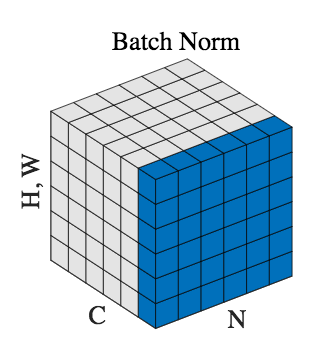
Statistics are computed for a whole batch, channel per channel.
$\gamma$ and $\beta$ are essential because they enable the BN to represent the identity transform if needed. If it couldn’t, the resulting BN’s transformation (with a mean of 0 and a variance of 1) fed to a sigmoid non-linearity would be constrained to its linear regime.
While during training the mean and standard deviation are computed on the batch, during test time BN uses the whole dataset statistics using a moving average/std.
Batch Normalization has showed a considerable training acceleration to existing architectures and is now an almost de facto layer. It has however for weakness to use the batch statistics at training time: With small batches or with a dataset non i.i.d it shows weak performance. In addition to that, the difference between training and test time of the mean and the std can be important, this can lead to a difference of performance between the two modes.
1.1. Batch ReNormalization
(Ioffe, 2017)’s Batch Renormalization (BR) introduces an improvement over Batch Normalization.
BN uses the statistics ($\mu_B$ & $\sigma_B$) of the batch. BR introduces two new parameters $r$ & $d$ aiming to constrain the mean and std of BN, reducing the extreme difference when the batch size is small.
Ideally the normalization should be done with the instance’s statistic:
$$\hat{x} = \frac{x - \mu}{\sigma}$$
By choosing $r = \frac{\sigma_B}{\sigma}$ and $d = \frac{\mu_B - \mu}{\sigma}$:
$$\hat{x} = \frac{x - \mu}{\sigma} = \frac{x - \mu_B}{\sigma_B} \cdot r + d$$
The authors advise to constrain the maximum absolute values of $r$ and $d$. At first to 1 and 0, behaving like BN, then to relax gradually those bounds.
1.2. Internal Covariate Shift?
Ioffe & Szegedy argued that the changing distribution of the pre-activation hurt the training. While Batch Norm is widely used in SotA research, there is still controversy (Ali Rahami’s Test of Time) about what this algorithm is solving.
(Santurkar et al, 2018) refuted the Internal Covariate Shift influence. To do so, they compared three models, one baseline, one with BN, and one with random noise added after the normalization.
Because of the random noise, the activation’s input is not normalized anymore and its distribution change at every time test.
As you can see on the following figure, they found that the random shift of distribution didn’t produce extremely different results:
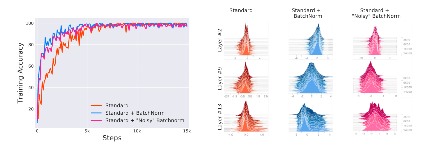
Comparison between standard net, net with BN, and net with noisy BN.
On the other hand they found that the Batch Normalization improved the Lipschitzness of the loss function. In simpler term, the loss is smoother, and thus its gradient as well.
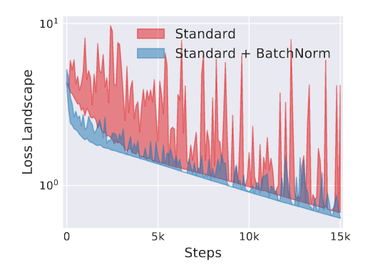
Figure 3: Loss with and without Batch Normalization.
According to the authors:
Improved Lipschitzness of the gradients gives us confidence that when we take a larger step in a direction of a computed gradient, this gradient direction remains a fairly accurate estimate of the actual gradient direction after taking that step. It thus enables any (gradient–based) training algorithm to take larger steps without the danger of running into a sudden change of the loss landscape such as flat region (corresponding to vanishing gradient) or sharp local minimum (causing exploding gradients).
The authors also found that replacing BN by a $l_1$, $l_2$, or $l_{\infty}$ lead to similar results.
2. Computing the mean and variance differently
Algorithms similar to Batch Norm have been developed where the mean & variance are computed differently.
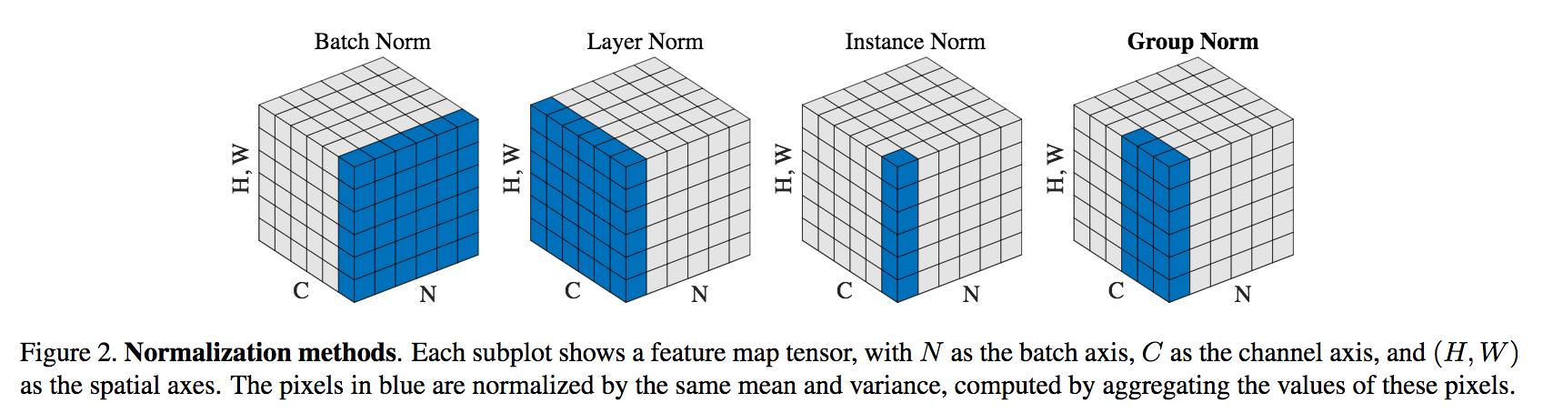
2.1. Layer Normalization
(Ba et al, 2016)’s layer norm (LN) normalizes each image of a batch independently using all the channels. The goal is have constant performance with a large batch or a single image. It’s used in recurrent neural networks where the number of time steps can differ between tasks.
While all time steps share the same weights, each should have its own statistic. BN needs previously computed batch statistics, which would be impossible if there are more time steps at test time than training time. LN is time steps independent by simply computing the statistics on the incoming input.
2.2. Instance Normalization
(Ulyanov et al, 2016)’s instance norm (IN) normalizes each channel of each batch’s image independently. The goal is to normalize the constrast of the content image. According to the authors, only the style image contrast should matter.
2.3. Group Normalization
According to (Wu and He, 2018), convolution filters tend to group in related tasks (frequency, shapes, illumination, textures).
They normalize each image in a batch independently so the model is batch size independent. Moreover they normalize the channels per group arbitrarily defined (usually 32 channels per group). All filters of a same group should specialize in the same task.
3. Normalization on the network
Previously shown methods normalized the inputs, there are methods were the normalization happen in the network rather than on the data.
3.1. Weight Normalization
(Salimans and Kingma, 2016) found that decoupling the length of the weight vectors from their direction accelerated the training.
A fully connected layer does the following operation:
$$y = \phi(W \cdot x + b)$$
In weight normalization, the weight vectors is expressed the following way:
$$W = \frac{g}{\Vert V \Vert}V$$
$g$ and $V$ being respectively a learnable scalar and a learnable matrix.
3.2. Cosine Normalization
(Luo et al, 2017) normalizes both the weights and the input by replacing the classic dot product by a cosine similarity:
$$y = \phi(\frac{W \cdot X}{\Vert W \Vert \Vert X \Vert})$$
4. Conclusion
Batch normalization (BN) is still the most represented method among new architectures despite its defect: the dependence on the batch size. Batch renormalization (BR) fixes this problem by adding two new parameters to approximate instance statistics instead of batch statistics.
Layer norm (LN), instance norm (IN), and group norm (GN), are similar to BN. Their difference lie in the way statistics are computed.
LN was conceived for RNNs, IN for style transfer, and GN for CNNs.
Finally weigh norm and cosine norm normalize the network’s weight instead of simply the input data.
EDIT: this post has been recommended by FastAI!