This post contains the notes taken from reading of the following paper:
This paper, published in 2012, describes an algorithm generating multiple possible object locations that will later be used by object recognition models. Fast-RCNN uses the Selective Search in its object proposal module.
Motivations
The authors divide the domain of object recognition in three categories:
- Exhaustive Search
- Segmentation
- Other sampling strategies (using Bag-of-Words, Hough Transform, etc.)
An Exhaustive Search tries to find bounding boxes for every objects in an image. Searching at every position and scale is unpracticable. Some use instead a windows of different ratio and make them slide around the image. More sophisticated methods also exists (1, 2).
Segmentation colors each pixel to a given class, creating objects with non-rigid shapes. Segmentation methods usually rely on a single strong algorithm to identify pixels’ regions.
Selective Search uses the best of both worlds: Segmentation improve the sampling process of different boxes. This reduces considerably the search space. To improve the algorithm’s robustness (to scale, lightning, textures…) a variety of strategies are used during the bottom-up boxes’ merging.
Selective Search produces boxes that are good proposals for objects, it handles well different image conditions, but more important it is fast enough to be used in a prediction pipeline (like Fast-RCNN) to do real-time object detection.
The Algorithm
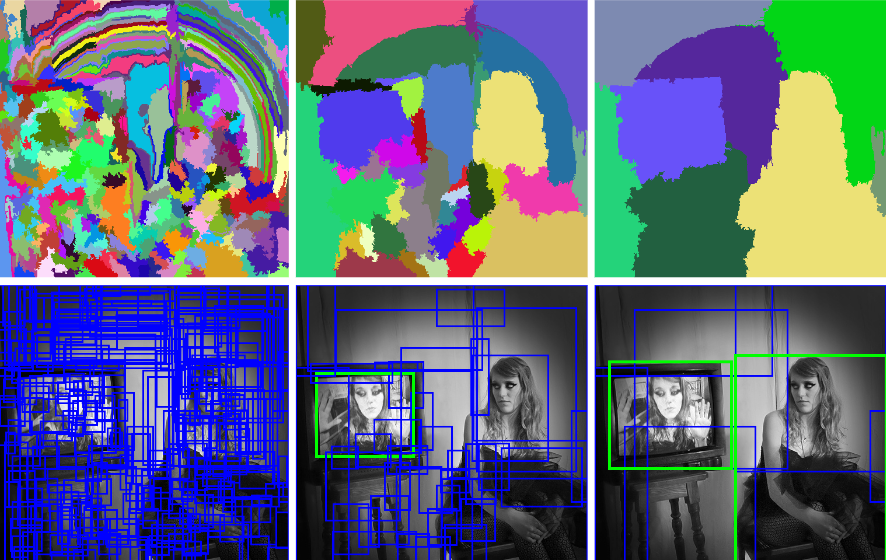
At first the authors produce a sampling a bounding boxes based on regions’ segmentation produced by the Efficient Graph-Based Segmentation.
Starting from these initial boxes, the authors use a bottom-up merging based on similarity: Boxes, small at first, are merged with their most similar neighbour box. The history of all seen boxes at the different steps of the algorithm is kept.

By keeping all existing boxes, the search can capture all scales which is important in hierarchical image: Imagine a pilot in a plane: the pilot’s box in comprised in the bigger plane’s box.
Plenty of boxes are created, the last box is the entire image! However some may be more probable object location. The authors sort the boxes by creation time, the most recent first. To avoid privileging too much large boxes, the box’s index (1 being the most recent box) is multiplied by a random number between 0 and 1.
![]()
The model using the selective search can now make a trade-off between having all location proposals and getting only the k-first most probable.
Diversification Strategies
The authors use three strategies to improve the search’s robustness:
1. Different color spaces
In order to handle different lightning, the authors apply their algorithm to the same image transposed in different color spaces.
The most known color space is RGB, where a pixel has values of red, blue, and green. Among the other used color spaces there are:
- Grayscale: Where a pixel has for single value its intensity.
- Lab: With one value for lightness, one for green-red, and one for blue-yellow.
- HSV: With hue, saturation, and a value
- etc.
2. Different Starting Regions
As said before, the algorithm produces its initial boxes from the regions generated by the efficient graph-based segmentation. This segmentation has a parameter $k$ that affects the size of the regions.
Different starting regions from the segmentation affect deeply the selective search.
3. Different Similarity Measures
The most interesting part of this algorithm is the different metrics used to assess similarity between boxes.
Four similarity measures are defined: Color, texture, size, fitness. These metrics are based on features computed with the pixels’ values. It would be slow to re-compute these features each time boxes are merged. The authors designed these features so that they could be merged and propagated to the new box without re-computing everything.
These similarities are added together producing a final similarity measure.
3.1. Color Similarity
Each box has a color histogram of 25 bins. The similarity of two boxes is the histogram intersection:
$$s_{color}(r_i, r_j) = \sum_{k=1}^n min(c^k_i, c^k_j)$$
With $r_x$ being a region, and $c^k$ a bin of the histogram.
It is simply the number of common pixel values:

To propagate the histogram to the box created by a merge of two smaller boxes, the authors average the two histograms with a size’s weight:
$$C_t = \frac{size(r_i) * C_i + size(r_j) * C_J}{size(r_i) + size(r_j)}$$
3.2. Texture Similarity
Textures matter a lot, otherwise how to make a difference between a cameleon and the material it sits on?
The authors create a texture histogram with SIFT. From this histogram, they use the same formulas for both histogram intersection and hierarchy propagation.
3.3. Size Similarity
The size similarity has been created in order to avoid an imbalance between the boxes’ size. Where one growing big box would forbid intermediary boxes to form.
$$s_{size}(r_i, r_j) = 1 - \frac{size(r_i) + size(r_j)}{size(image)}$$
The propagation of this feature is simply the sum of the two sizes.
3.4. Fitness Feature
The initial boxes created from the segmentation may overlap. Two overlapping boxes should be merged early, to do this a fitness feature is used:
$$s_{\text{fitness}}(r_i, r_j) = 1 - \frac{size(BB_{ij} - size(r_i) - size(r_j))}{size(\text{image})}$$
The box $BB_{ij}$ is a bounding box that contains both $r_i$ and $r_j$. The feature $s_{\text{fitness}}$ is proportional to the fraction covered by $r_i$ and $r_j$ in the bounding box $BB_{ij}$.
Exploiting The Search
Creating bounding boxes is interesting. However the end goal here is to use the selective search in a object recognition model.
The authors use a SVM with an histogram intersection kernel. SVMs are binary classifiers (but can be expanded to multi-classification with One-Against-Rest, One-Against-All schemes). The positive bounding boxes are ground-truth objects. The negative bounding boxes are boxes generated by the selective search that have an overlap of 20% to 50% with a positive box. This force the SVMs to train on particularly difficult boxes.
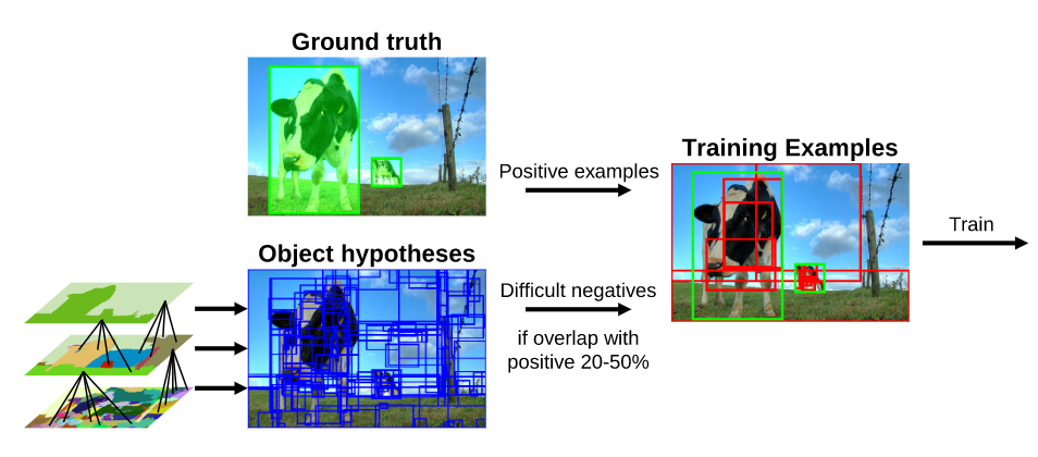
However SVMs are slow to train with large amount of data. I will publish another article on Fast-RCNN, a model that use Convolutional Neural Networks on top of the Selective Search to do object recognition.