This article contains note of the research paper:
- Densely Connected Convolutional Networks by Cornell Uni, Tsinghua Uni, and Facebook Research.
This paper was awarded the CVPR 2017 Best Paper Award.
Introduction
DenseNet is a new CNN architecture that reached State-Of-The-Art (SOTA) results on classification datasets (CIFAR, SVHN, ImageNet) using less parameters.
Thanks to its new use of residual it can be deeper than the usual networks and still be easy to optimize.
General Architecture
DenseNet is composed of Dense blocks. In those blocks, the layers are densely connected together: Each layer receive in input all previous layers output feature maps.
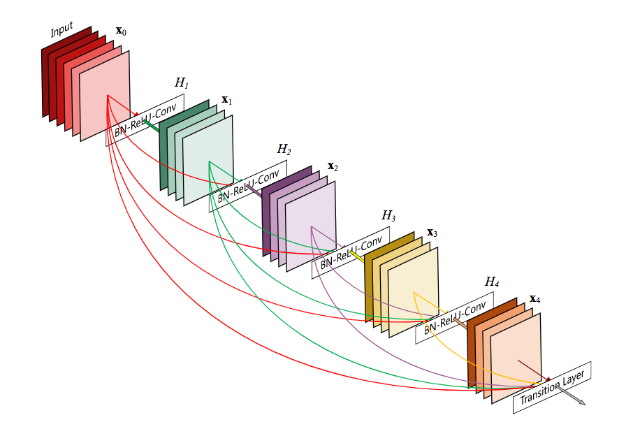
This extreme use of residual creates a deep supervision because each layer receive more supervision from the loss function thanks to the shorter connections.
1. Dense block
A dense block is a group of layers connected to all their previous layers. A single layer looks like this:
- Batch Normalization
- ReLU activation
- 3x3 Convolution
The authors found that the pre-activation mode (BN and ReLU before the Conv) was more efficient than the usual post-activation mode.
Note that the authors recommend a zero padding before the convolution in order to have a fixed size.
2. Transition layer
Instead of summing the residual like in ResNet, DenseNet concatenates all the feature maps.
It would be impracticable to concatenate feature maps of different sizes (although some resizing may work). Thus in each dense block, the feature maps of each layer has the same size.
However down-sampling is essential to CNN. Transition layers between two dense blocks assure this role.
A transition layer is made of:
- Batch Normalization
- 1x1 Convolution
- Average pooling
Growth rate
Concatenating residuals instead of summing them has a downside when the model is very deep: It generates a lot of input channels!
You may now wonder how could I say in the introduction that DenseNet has less parameters than an usual SotA networks. There are two reasons:
First of all a DenseNet’s convolution generates a low number of feature maps. The authors recommend 32 for optimal performance but shows SotA results with only 12 output channels!
The number of output feature maps of a layer is defined as the growth rate.
DenseNet has lower need of wide layers because as layers are densely connected there is little redundancy in the learned features. All layers of a same dense block share a collective knowledge.
The growth rate regulates how much new information each layer contributes to the global state.
Bottleneck
The second reason DenseNet has few parameters despite concatenating many residuals together is that each 3x3 convolution can be upgraded with a bottleneck.
A layer of a dense block with a bottleneck will be:
- Batch Normalization
- ReLU activation
1x1 Convolution bottleneck producing: $\text{grow rate} * 4$ feature maps.
Batch Normalization
ReLU activation
3x3 Convolution
With a growth rate of 32, the tenth layer would have in input 288 feature maps! Thanks to the bottleneck at most 128 feature maps would be fed to a layer. This helps the network have hundred, if not thousand, layers.
Compression
The authors further improves the compactness of the model with a compression. This compression happens in the transition layer.
Normally the transition layer’s convolution does not change the number of feature maps. In the case of the compression, its number of output feature maps is $\theta * m$. With $m$ the number of input feature maps and $\theta$ a compression factor between 0 and 1.
Note that the compression factor $\theta$ has the same role as the parameter $\alpha$ in MobileNet.
Conclusion
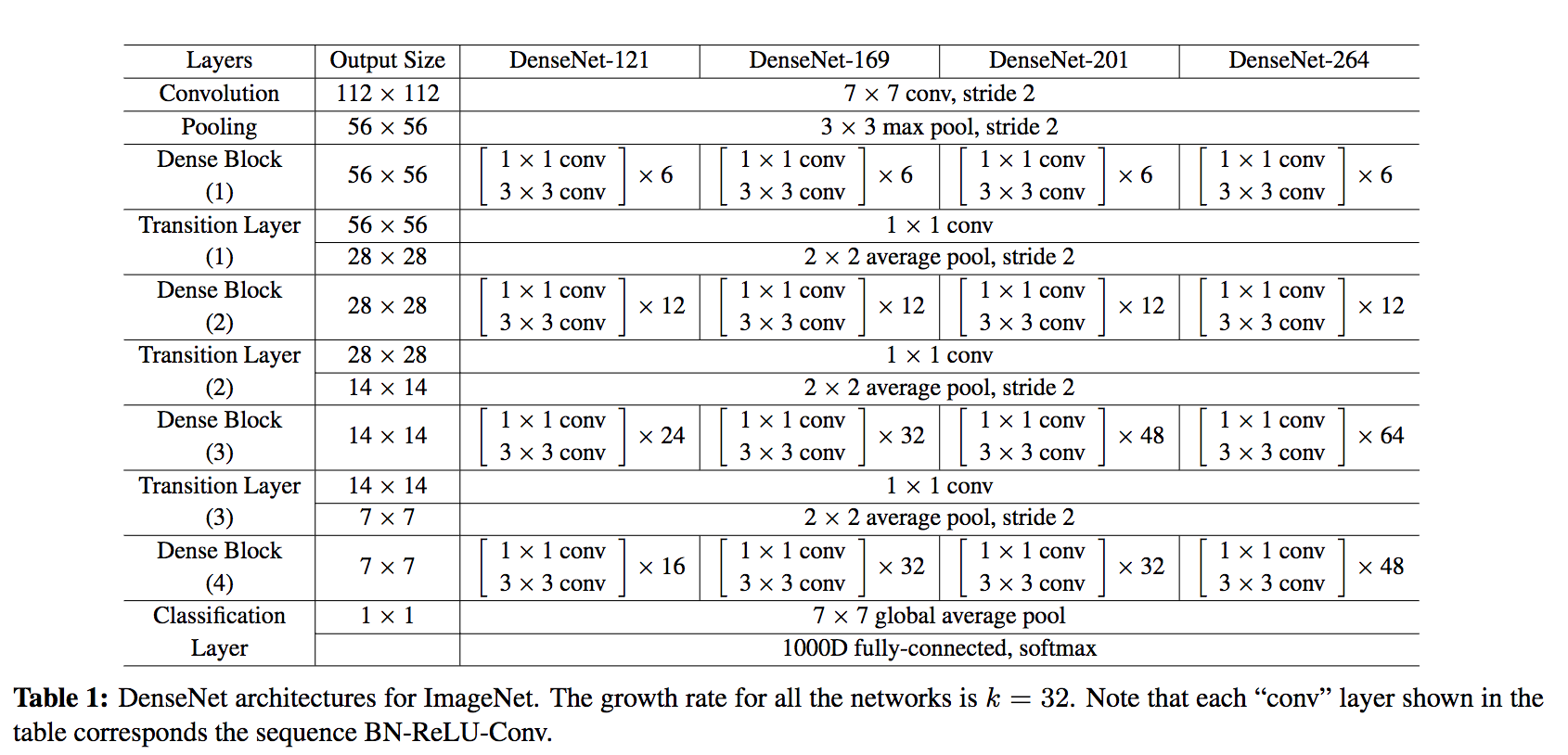
The final architecture of DenseNet is the following:
To summarize, the DenseNet architecture uses the residual mechanism to its maximum by making every layer (of a same dense block) connect to their subsequent layers.
This model’s compactness makes the learned features non-redundant as they are all shared through a common knowledge.
It is also far more easy to train deep network with the dense connections because of an implicit deep supervision where the gradient is flowing back more easily thanks to the short connections.