This post contains the notes taken from the following paper:

• Fast-RCNN by R. Girshick.

• Faster-RCNN by Microsoft Research.

Ross Girshick is an influential researcher on object detection: he has worked on RCNN, Fast{er}-RCNN, Yolo, RetinaNet…

Fast-RCNN and Faster-RCNN are both incremental improvements on the original RCNN.

Let’s see what were those improvements:

Fast-RCNN

In Fast-RCNN, Girshick ditched the SVM used previously. It resulted in a 10x inference speed improvement, and a better accuracy.

Girshick replaced the SVM by a Region of Interest (RoI) pooling. RoIs are still produced by the selective search, and they are used to select a subset of the feature map produced from the whole image:

At the end of the CNN, without top, a feature map is generated by filter.

Let’s consider as example an input image of size 10x10; At the end of the CNN, the feature map has a size of 5x5. If the selective search proposes a box between (top-left and bottom-right) (0, 2) and (6, 8) then we extract a similar box from the feature map. However this box is proportionally scaled down:

Objects have different sizes, and so are the boxes extracted from the feature maps. To normalize their size a max pooling is done. Note that it does not really matter if the height or width of the extracted box is not even:

Those extracted fixed-size feature maps (one per filter per object) are then fed to fully connected layers. At some point, the network split into two sub-networks. One is designed to classify the class with a softmax activation. The other is a regressor with 4 values: The coordinates of the top-left point of the box and its width & height.

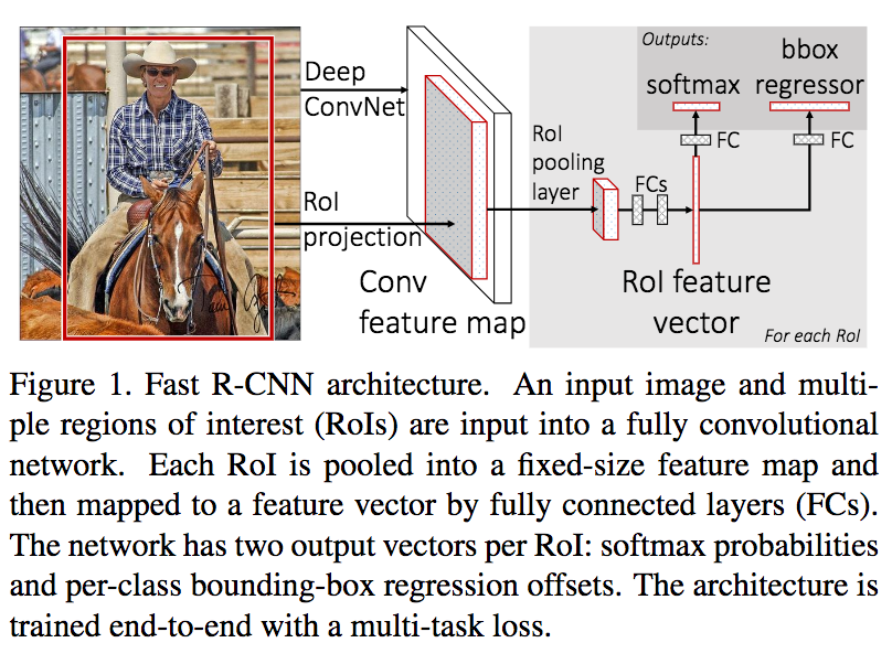
Note that if you want to train your RCNN to detect $K$ classes, the sub-network detecting the box’s class will choose between $K + 1$ classes. The extra class is the ubiquitous background. The bounding-box regressor’s loss won’t be taken in account if a background is detected.

Faster-RCNN

The main contribution of Fast-RCNN was the RoI pooling followed by a two-headed fully connected network. Faster-RCNN eliminated another speed bottleneck: The generation of the region proposals by selective search:

Fast R-CNN, achieves near real-time rates using very deep networks, when ignoring the time spent on region proposals. Now, proposals are the test-time computational bottleneck in state-of-the-art detection systems.

The authors introduced the Region Proposal Network (RPN) to fix this problem.

Region Proposal Network

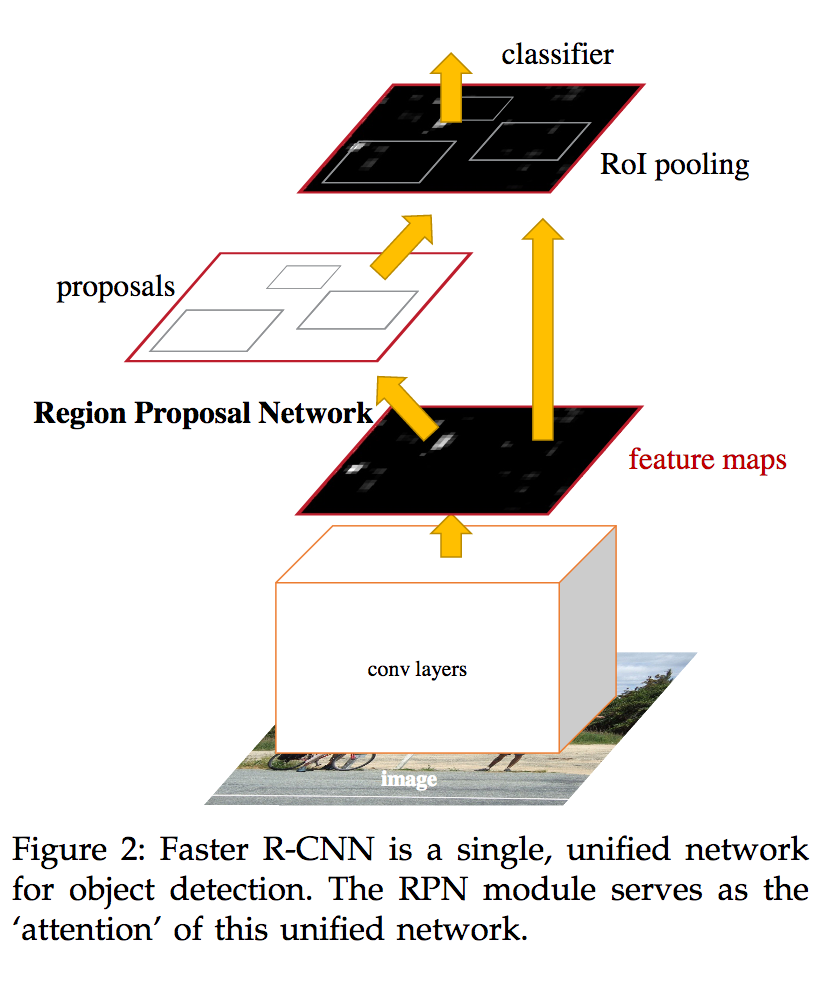RPN generates region proposals that are given to the classifier which is Fast-RCNN.

First of all the feature maps are reduced to intermediate layers of smaller size. The authors used a layer of dimension 512 when the feature maps were originating from VGG16.

Then the RPN uses a sliding window, moving all around the intermediate layers. At each location, anchors are used. An anchor is simply a box of a pre-defined size and shape. 9 different anchors exist: there are 3 different scales and 3 different ratios.

The first two scales, and the three possible ratios.

For each possible anchor a mini-network is used for two tasks:

• classify whether the location is a background or an actual object.
• Predict the exact bounding-box coordinates and width.

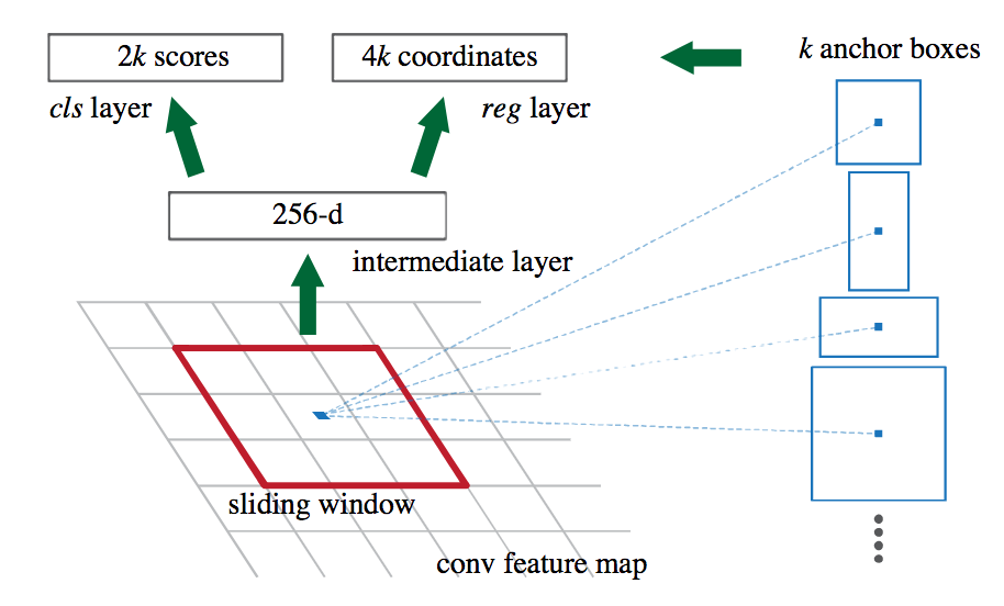With $k = 9$, the number of anchor.

Finally these object proposals are fed to the same top as Fast-RCNN.

How to Train

In addition of the RPN, I’ve really found interesting how the authors used tricks to train their model.

A big problem of object detection model is that most of the proposal are coming from background (RetinaNet solves this problem elegantly). The authors sample 256 proposals for an image where background and non-background proposals are in equal quantity. The loss function is computed on this sampling.

The features of Fast-RCNN and the RPN are shared. To take advantage of this, the authors tried four training strategies:

• Alternate sharing: Similar to some matrix decomposition methods, the authors train RPN, then Fast-RCN, and so on. Each network is trained a bit alternatively.

• Approximate joint training: This strategy consider the two networks as a single unified one. The back-propagation uses both the Fast-RCNN loss and the RPN loss. However the regression of bounding-box coordinates in RPN is considered as pre-computed, and thus its derivative is ignored.

• Non-approximate joint training: This solution was not used as more difficult to implement. The RoI pooling is made differentiable w.r.t the box coordinates using a RoI warping layer.

• 4-Step Alternating training: The strategy chosen takes 4 steps: In the first of one the RPN is trained. In the second, Fast-RCNN is trained using pre-computed RPN proposals. For the third step, the trained Fast-RCNN is used to initialize a new RPN where only RPN’s layers are fine-tuned. Finally in the fourth step RPN’s layers are frozen and only Fast-RCNN is fine-tuned.

Summary

These two papers are incremental improvements of RCNN. They introduce RoI pooling and Region Proposal Network.

RoI pooling concept is also used in other models. FashionNet, a model to predict clothes’ attributes uses a concept of landmark pooling to force model’s attention on a particular cloth’s trait.

Region Proposal Network is now used in most object detection models, like the Feature Pyramid Network.