Imagine you’re in a landlocked country, and an infection has spread. The government has fallen, and rebels are roaming the country. If you’re the armed forces in this scenario, how do you make decisions in this environment? How can you fully understand the situation at hand?

A few weeks ago, NATO organized an innovation challenge that posed these questions. We decided to take on the challenge with the goal of finding innovative solutions in the areas of data filtering/fusing, visualization, and predictive analytics.
For those who don’t know, NATO is an intergovernmental military alliance between 29 North American and European countries. It constitutes a system of collective defense whereby its independent member states agree to mutual defense in response to an attack by any external party.
NATO did not provide any data for the challenge, so we had to find it ourselves. Ultimately, the solution we came up with used a variety of different techniques including computer vision on aerial imagery, natural language processing on press & social media, geo data processing, and — of course — fancy graphs.
In this post, we will focus on the most technical part: object detection for aerial imagery, walking through what kind of data we used, which architecture was employed, and how the solution works, and finally our results. If you’re interested in a higher-level look at the project, that’s over here.
This challenge was done while I was an intern at Dataiku. My team was composed of an commander, a salesman, and myself as the lead/sole scientist.
1. The dataset
For the object detection portion of the project, we used the Cars Overhead With Context (COWC) dataset, which is provided by the Lawrence Livermore National Laboratory. It features aerial imagery taken in six distinct locations:
- Toronto, Canada
- Selwyn, New Zealand
- Potsdam and Vaihingen*, Germany
- Columbus (Ohio)* and Utah, USA
* We ultimately did not use the Columbus and Vaihingen data because the imagery was in grayscale.
This dataset offers large imagery (up to 4 square kilometers) with good resolution (15cm per pixel) with the center localization of every car. As suggested in this Medium post, we assumed that cars have a mean size of 3 meters. We created boxes centered around each car center to achieve our ultimate goal of predicting box (i.e., car) locations in unseen images.
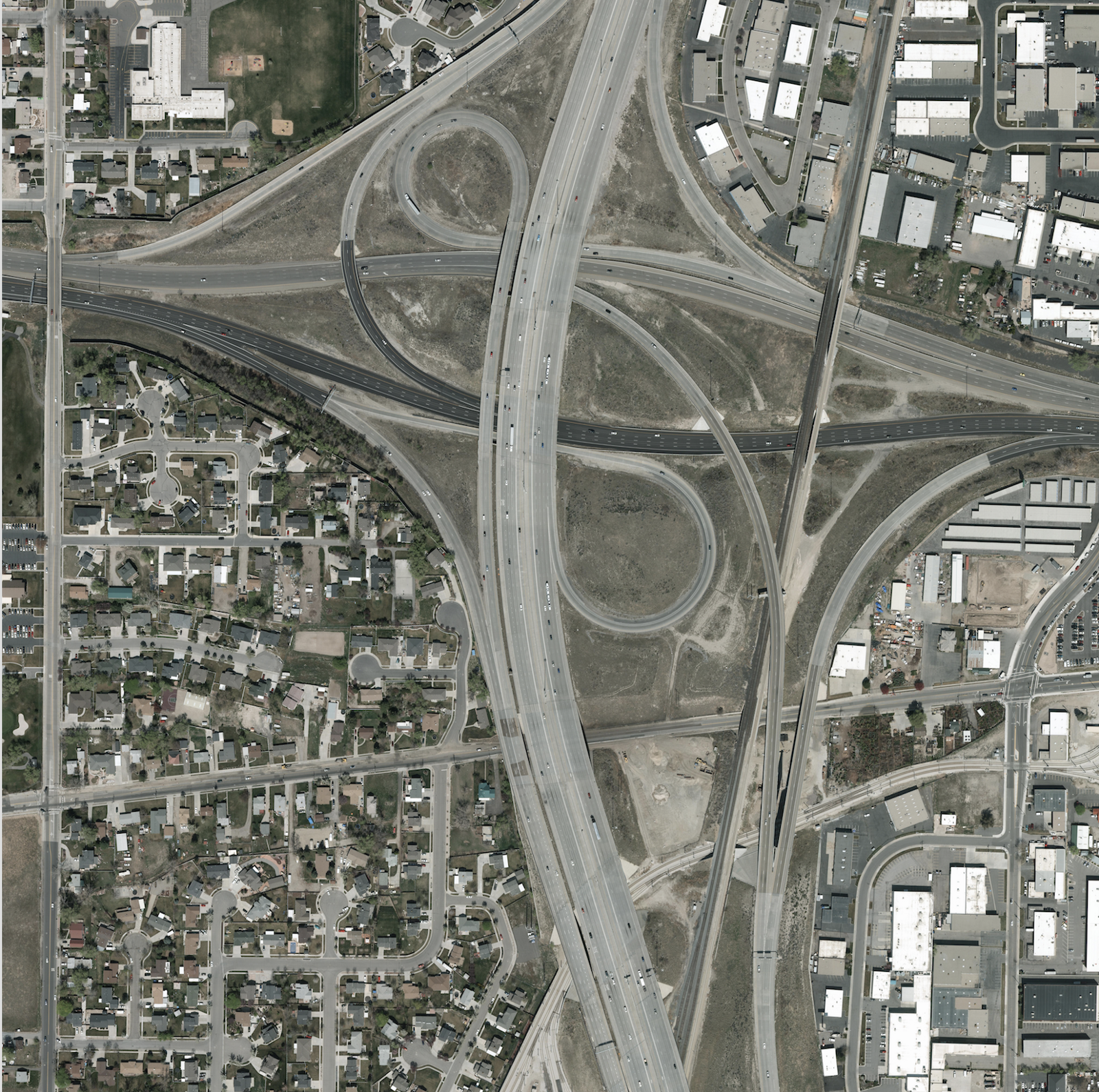
Figure 1: An example image from the COWC dataset
2. The architecture
To detect cars in these large aerial images, we used the RetinaNet (Lin et al, 2017) architecture. Published in 2017 by Facebook FAIR, this paper won the Best Student Paper of ICCV 2017.
Object detection architectures are split in two categories: single-stage and two-stage.
Two-stage architectures first categorize potential objects in two classes: foreground or background. Then all foreground’s potential objects are classified in more fine-grained classes: cats, dogs, cars, etc. This two-stage method is slow but also, and of course, produces the best accuracy. The most famous two-stage architecture is Faster-RCNN (Ren et al, 2015).
On the other hand, single-stage architectures don’t have this pre-selection step of potential foreground objects. They are usually less accurate, but they are also faster. RetinaNet’s single-stage architecture is an exception: it reaches two-stage performance while having single-stage speed!
On the figure 2 below, you can see a comparison of object detection architectures.
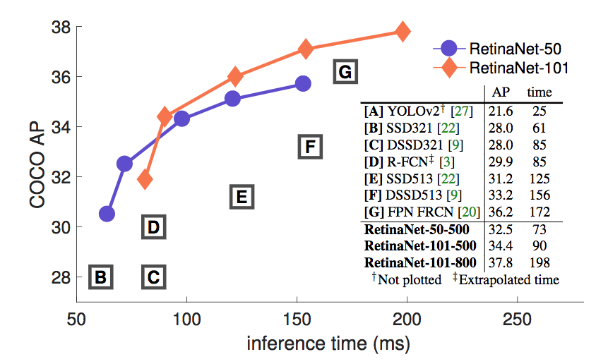
Figure 2: Performance of object detection algorithms
RetinaNet is made of four components. We’ll try to describe how the data is transformed through every step.

Figure 3: The RetinaNet architecture
2.1. Convolutional Network
First of all there is a ResNet-50 (He et al., 2015). As every convolutional neural network (CNN), it takes an image as input and processes it through convolution kernels. Each kernel’s output is a feature map — the first feature maps capture high-level features (such as a line or a color). The further we go down in the network, the smaller the feature maps become because of the pooling layers. While they are smaller, they also represent more fined-grained information (such as an eye, a dog ear, etc.). The input image has three channels (red, blue, green), but every subsequent feature map has dozens of channels! Each of them represents a different kind of feature that it captured.
A common classifier takes the ResNet’s last feature maps (of shape (7, 7, 2048)),
applies an average pooling on each channel (resulting in (1, 1, 2048)), and feeds
it to a fully connected layer with a softmax.
2.2. Feature Pyramid Network
Instead of adding a classifier after ResNet, RetinaNet adds a Feature Pyramid Network (FPN) (Lin et al., 2016). By picking feature maps at different layers from the ResNet, it provides rich and multi-scale features.
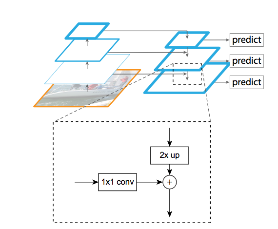
Figure 4: The lateral connection between the backbone and the FPN
However, ResNet’s first feature maps may be too crude to extract any useful information. As you can see in figure 4, the smaller and more precise feature maps are combined with the bigger feature maps. We first upsample the smaller ones and then sum it with the bigger ones. Several upsampling methods exist; here, the upsampling is done with the nearest neighbor method.
Each level of the FPN encodes a different kind of information at a different scale. Thus, each of them should participate in the object detection task. The FPN takes as input the output of the third (512 channels), fourth (1024 channels), and fifth (2048 channels) blocks of ResNet. The third is half the size of the fourth, and the fourth is half of the fifth.
We apply pointwise convolution (convolution with a 1x1 kernel) to uniformize the number of channels of each level to 256. Then we upsampled the smaller levels by a factor of two to match the dimension of the bigger levels.
2.3. Anchors
At each FPN level, anchors are moved around the FPN’s feature maps. An anchor is a rectangle with different sizes and ratios, like this:
Figure 5: A sample of anchors of different sizes and ratios
These anchors are the base position of the potential objects. Five sizes and three ratios exist, thus there are 15 unique anchors. These anchors are also scaled according to the dimension of the FPN levels. These unique anchors are duplicated on all the possible positions in the feature maps. It results in $K$ total anchors.
Let’s put aside those anchors for the moment.
2.4. Regression & classification
Each FPN’s level is fed to two Fully Convolutional Networks (FCN), which are neural networks made only of convolutions and pooling. To fully exploit the fact that every FPN’s level holds different kind of information, the two FCNs are shared among all levels! Convolution layers are independent of the input size; only their kernel size matter. Thus while each FPN’s feature maps have different sizes, they can be all fed to the same FCNs.
The first FCN is the regression branch. It predicts $K x 4$
(x1, y1, x2, y2 for each anchor) values. Those values are deltas that
slightly modify the original anchors so they fit the potential objects
better. All the potential objects will now have coordinates of the type:
(x1 + dx1, y1 + dy1, x2 + dx2, y2 + dy2)
With x? and y?, the fixed coordinates of the anchors, and dx?, dy?,
the deltas produced by the regression branch.
We now have the final coordinates for all objects — that is, all potential objects. They are not yet classified as background or car, truck, etc.
The second FCN is the classification branch. It is a multi-label problem where the classifier predicts $K x N$ ($N$ being the number of classes) potential objects with sigmoid.
2.5. Removing duplicates
At this point we have $K x 4$ coordinates and $K x N$ class scores. We now have a problem: it is common to detect, for the same class, several boxes for a same object!
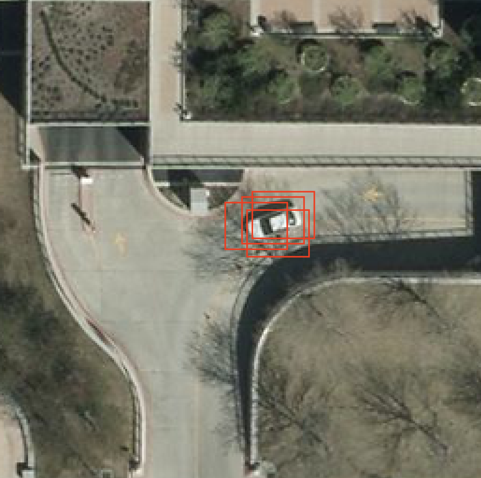
Figure 6: Several boxes have been detected for a single car.
Therefore, for each class (even if it’s not the highest scoring class) we apply a Non-max suppression. Tensorflow provides a function to do it:
tf.image.non_max_suppression(boxes, scores, max_output_size, iou_threshold)The main gist of this method is that it will remove overlapping boxes
(such as in Figure 6) to keep only one. It also using the scores to keep the
most probable box.
A general comment on the input parameter of the Tensorflow method above:
The max_output_size corresponds to the maximum number of boxes we want at the
end — let’s say 300. The iou_threshold is a float between 0 and 1, describing
the maximum ratio of overlapping that is accepted.
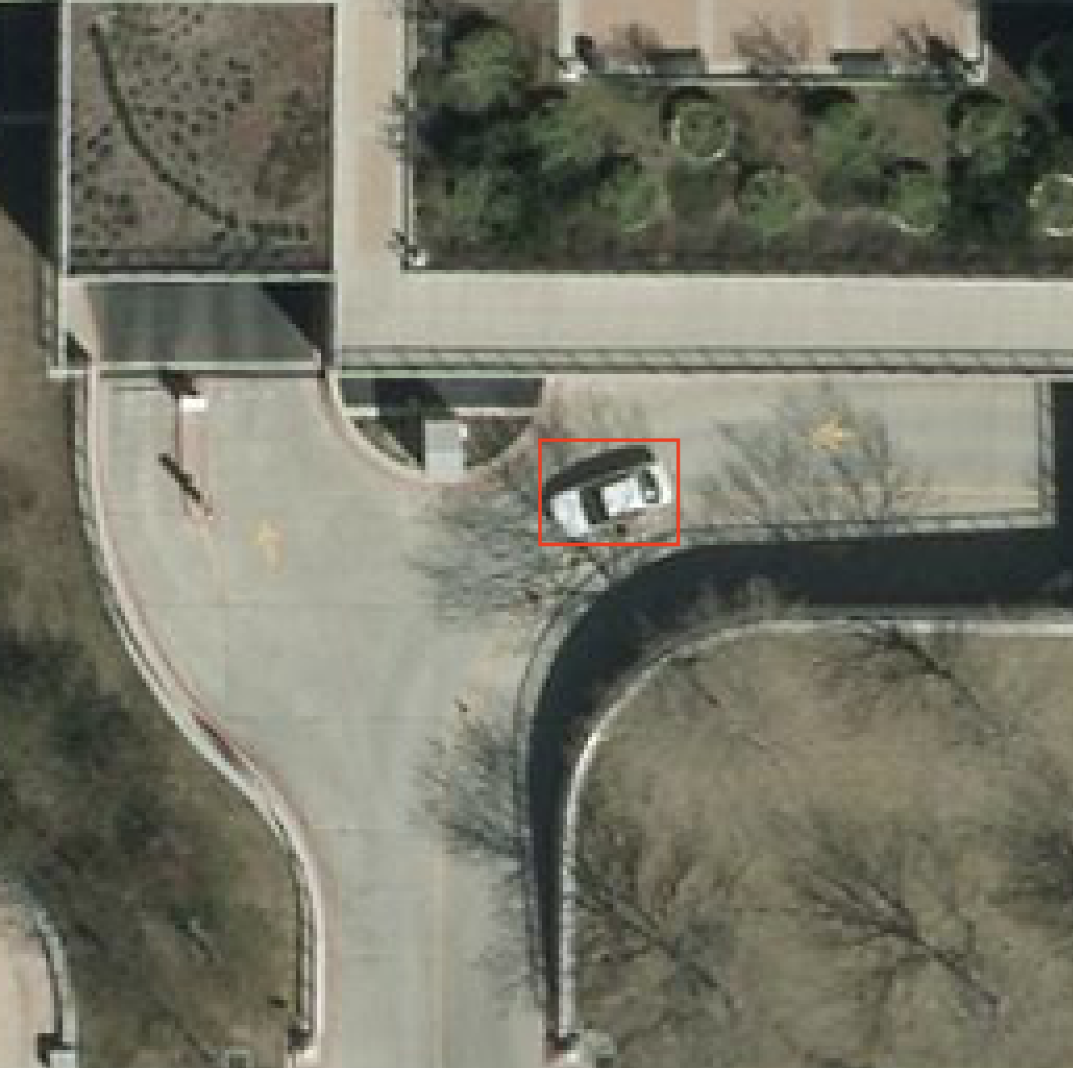
Figure 7: Figure 6 after the non-max-suppression has been applied.
2.6. Keeping the most probable class
Duplicate boxes for the same class at the same place are now removed. For each of the remaining boxes, we are keeping only the highest-scoring class (car, truck, etc.). If none of the classes have a score above a fixed threshold (we used $0.4$), it’s considered to be part of the background.
2.7. The Focal Loss
All this may sound complicated, but it’s nothing new — it’s not enough to have good accuracy. The real improvement from RetinaNet is its loss: the Focal Loss. Single-stage architectures that don’t have potential objects pre-selection are overwhelmed with the high frequency of background objects. The Focal Loss deals with it by according a low weight to well-classified examples, usually the background.

Figure 8: We define Pt, the confidence to be right
In Figure 8, we define $p_t$, the confidence to be right in a binary classification.

Figure 9: The Focal Loss
In Figure 9, we module the cross entropy loss $-\log(p_t)$ by a factor $(1 — p_t)^\gamma$. Here, $\gamma$ is a modulating factor oscillating between 0 and 5. The well-classified examples have a high $p_t$ , and thus a low factor. Therefore, the loss for well-classified examples is low and forces the model learn on harder examples. You can see in Figure 10 how much the loss is affected.
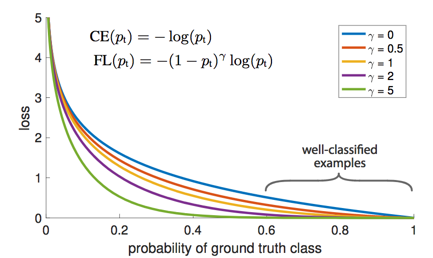
Figure 10: The focal loss under various modulating factors
3. Implementation
We used the excellent Keras implementation of RetinaNet by Fizyr. We also wrote a new generator, taking Pandas’ DataFrames instead of CSV files.
class DfGenerator(CSVGenerator):
    def __init__(self, df, class_mapping, cols, base_dir='', **kwargs):
        """Custom generator intended to work with in-memory Pandas' dataframe.

        Arguments:
            df: Pandas DataFrame containing paths, labels, and bounding boxes.
            class_mapping: Dict mapping label_str to id_int.
            cols: Dict Mapping 'col_{filename/label/x1/y1/x2/y2} to corresponding df col.
        """
        self.base_dir = base_dir
        self.cols = cols
        self.classes = class_mapping
        self.labels = {v: k for k, v in self.classes.items()}

        self.image_data = self._read_data(df)
        self.image_names = list(self.image_data.keys())

        Generator.__init__(self, **kwargs)

    def _read_classes(self, df):
        return {row[0]: row[1] for _, row in df.iterrows()}

    def __len__(self):
        return len(self.image_names)

    def _read_data(self, df):
        data = {}
        for _, row in df.iterrows():
            img_file, class_name = row[self.cols['col_filename']], row[self.cols['col_label']]
            x1, y1 = row[self.cols['col_x1']], row[self.cols['col_y1']]
            x2, y2 = row[self.cols['col_x2']], row[self.cols['col_y2']]

            if img_file not in data:
                data[img_file] = []

            # Image without annotations
            if not isinstance(class_name, str) and np.isnan(class_name):
                continue

            data[img_file].append({
                'x1': int(x1), 'x2': int(x2),
                'y1': int(y1), 'y2': int(y2),
                'class': class_name
            })

return data
As you can see, images without annotations are kept in the training phase. They still help the training of our algorithm, as it forces the algorithm to not see cars everywhere (even where there aren’t any).
We used a pre-trained RetinaNet on COCO and then fine-tuned it for the COWC dataset. Only the two FCNs are retrained for this new task, while the ResNet backbone and the FPN are frozen.
You can see in the code block below how to load the RetinaNet and compile it.
Note that it is important to add skip_mismatch=True when loading the weights!
The weights were created on COCO with 80 classes, but in our case we only have
1 class, thus the number of anchors is not the same.
def load_retinanet(weights, n_classes, freeze=True):
    modifier = freeze_model if freeze else None

    model = resnet50_retinanet(num_classes=num_classes, modifier=modifier)
    model.load_weights(weights, by_name=True, skip_mismatch=True)

    return model


def compile(model):
    model.compile(
        loss={
            'regression'    : keras_retinanet.losses.smooth_l1(),
            'classification': keras_retinanet.losses.focal()
        },
        optimizer=optimizers.adam(lr=configs['lr'], clipnorm=0.001)
    )


def train(model, train_gen, val_gen, callbacks, n_epochs=20):
    """train_gen and val_gen are instances of DfGenerator."""
    model.fit_generator(
        train_gen,
        steps_per_epoch=len(train_gen),
        validation_data=val_gen,
        validation_steps=len(val_gen),
        callbacks=callbacks,
        epochs=n_epochs,
        verbose=2
)
There is something we still need to deal with, which is the massive weight of each image. Images from the COWC dataset are up to 4 square kilometers, or 13k pixel wide and high. Those big images weigh 300mb. It is impracticable to feed such large images to our RetinaNet. Therefore, we cut the images in patches of 1000x1000 pixels (or 150x150 meters).
However, it would be stupid to miss cars because they’d been cut between two patches. So to avoid this problem, we made a sliding window of 1000x1000 pixels that moves by steps of 800 pixels. That way, there is a 200-pixel-wide overlap between two adjacent patches.
This leads to another problem: we may detect cars twice. To remove duplicates, we applied non-max suppression when binding together the small patches. Indeed, that means we have a non-max suppression twice: after the RetinaNet and when binding together the small patches. For the second non-max suppression, we used a Numpy version of the algorithm. You can either use a fast & vectorized version by PyImageSearch, or the following naive version:
def jaccard(a, b):
    """Compute the jaccard score between box a and box b."""
    side1 = max(0, min(a[2], b[2]) - max(a[0], b[0]))
    side2 = max(0, min(a[3], b[3]) - max(a[1], b[1]))
    inter = side1 * side2

    area_a = (a[2] - a[0]) * (a[3] - a[1])
    area_b = (b[2] - b[0]) * (b[3] - b[1])

    union = area_a + area_b - inter

    return inter / union


def naive_nms(boxes, scores, threshold=0.4):
    scores_idx = scores.argsort()[::-1] # Keep highest scores first
    boxes = boxes[scores_idx]

    indices_to_skip = set()
    for i in range(boxes.shape[0]):
        for j in range(boxes.shape[0]):
            if i == j or j in indices_to_skip:
                continue

            if jaccard(boxes[i], boxes[j]) > threshold:
                indices_to_skip.add(j)

    mask = np.ones(boxes.shape[0], np.bool)
    mask[np.array(list(indices_to_skip))] = 0
    return boxes[mask]
When dealing with aerial imagery, we can use a lot of data augmentation. First of all, we can flip the horizontal axis and the vertical axis. We can also rotate the image by any angle. If the imagery’s scale is not uniform (the distance drone-to-ground may not be constant), it is also useful to randomly scale down and up the pictures.
4. Results
You can see on Figures 11 and 12 below how our RetinaNet behaves on this unseen image of Salt Lake City.
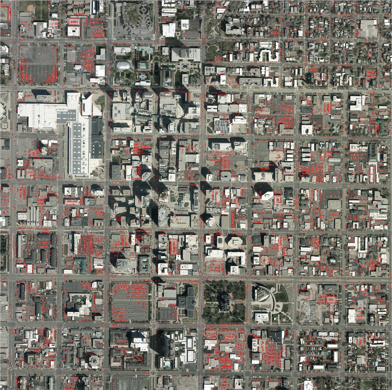
Figure 11: 13,000 detected cars in a 4 square kilometer area of Salt Lake City
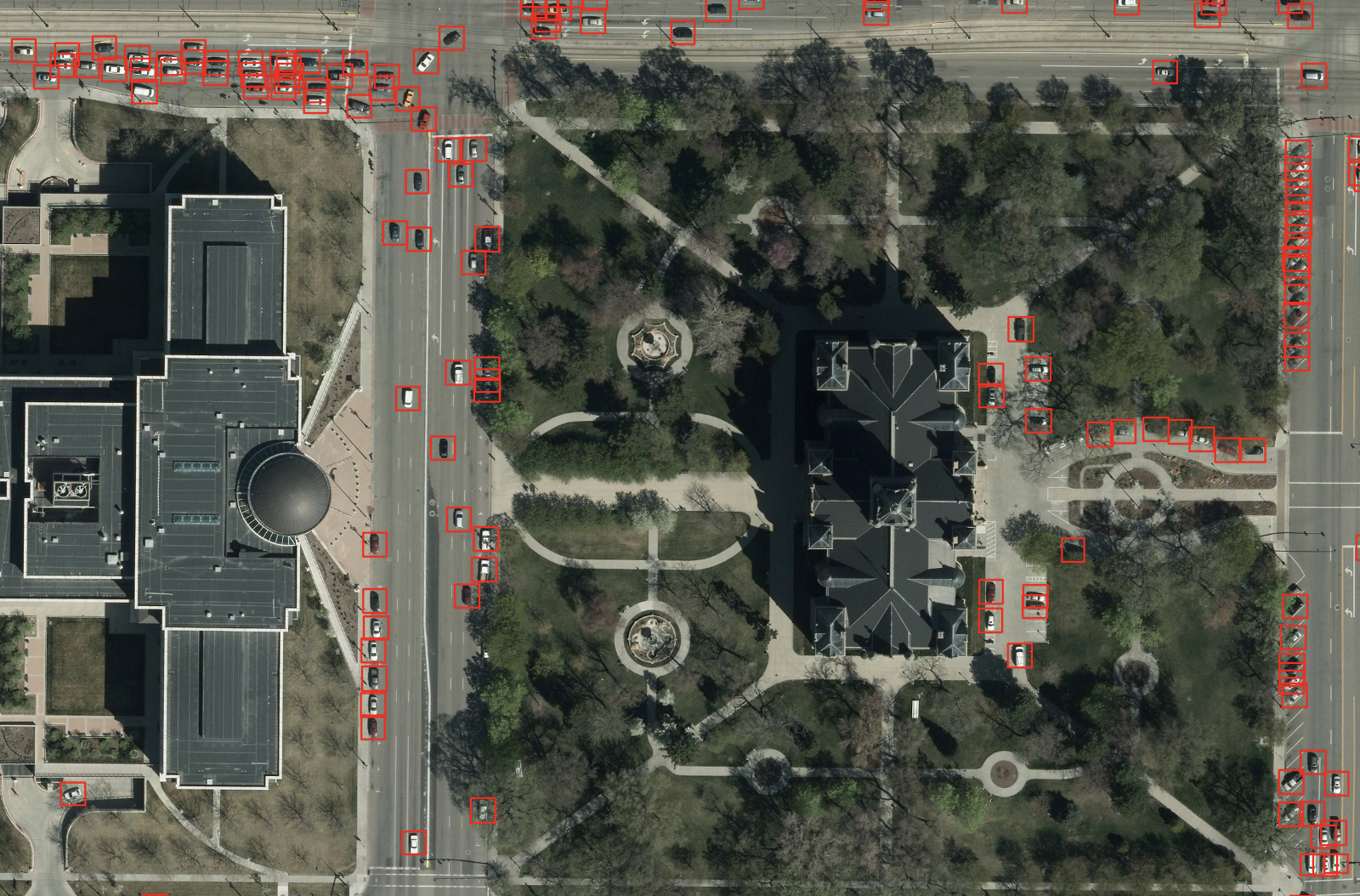
Figure 12: A zoom in of Figure 11
5. Are we good?
How can we evaluate our performance?
Accuracy is not enough; we need to see how many false positives and false negatives we get. If we detect cars everywhere, we’d have a lot of false positive, but if we miss most of the cars, that’s a lot of false negative.
The recall measures the former while the precision measures the latter. Finally, the f1-score is a combination of those two metrics.
def compute_metrics(true_pos, false_pos, false_neg):
    """Compute the precision, recall, and f1 score."""
    precision = true_pos / (true_pos + false_pos)
    recall = true_pos / (true_pos + false_neg)

    if precision == 0 or recall == 0:
        return precision, recall, 0

    f1 = 2 / (1 / precision + 1 / recall)
    return precision, recall, f1
However, we are not expecting our RetinaNet to detect the cars at the exact right pixels. Therefore, we are computing the Jaccard Index of the detected cars and the ground-truth cars, and if it is more than a chosen threshold, we consider that the car was rightfully detected. Note that the Jaccard index is often also (blandly) called Intersection-over-Union (IoU):
def jaccard(box_a, box_b):
    """box_X is a tuple of the shape (x1, y1, x2, y2)."""
    side1 = max(0, min(a[2], b[2]) - max(a[0], b[0]))
    side2 = max(0, min(a[3], b[3]) - max(a[1], b[1]))
    inter = side1 * side2

    area_a = (a[2] - a[0]) * (a[3] - a[1])
    area_b = (b[2] - b[0]) * (b[3] - b[1])
    union = area_a + area_b - inter

    return inter / union


def is_valid(box_pred, box_true, threshold=0.3):
    return jaccard(box_red, box_true) >= threshold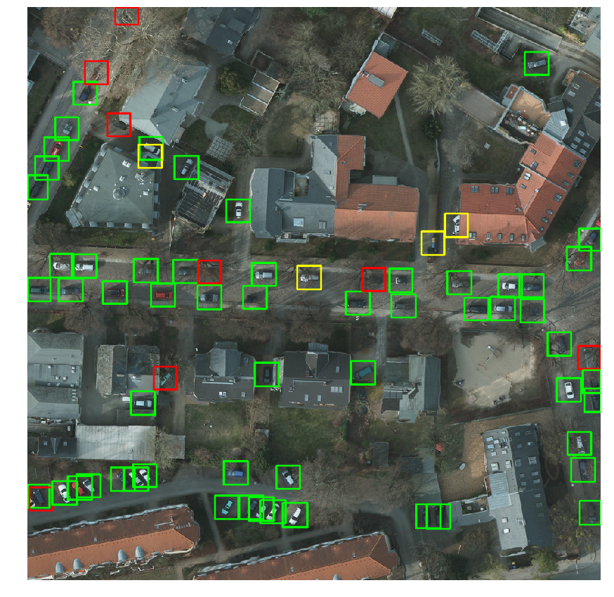
Figure 13: True Positive (green), False Positive (yellow), and False Negative (red)
You can see a sample on Figure 13 where true positives, false positives, and false negatives have been plotted.
Note that among the four false positives, two of them are garbage bins, one is a duplicate, and one is actually… a car! Indeed, as in every dataset, there may be some errors in the ground-truth annotations.
On Figure 12, the f1-score is $0.91$. Usually in more urban environments the f1-score is around $0.95$. The main mistake our model makes is considering ventilation shafts on tops of buildings to be cars. To the model’s defense, without knowledge of building, it’s quite hard to see that.
6. Conclusion
For the NATO challenge, we didn’t only use car detection from aerial imagery, but it was the main technical part of the project.
Oh… Did we forget to tell you the challenge results?
Three prizes were awarded: The NATO prize (with a trip to Norfolk), the France prize (with $25k), and the Germany prize (with a trip to Berlin).
We won both the NATO and France prize!
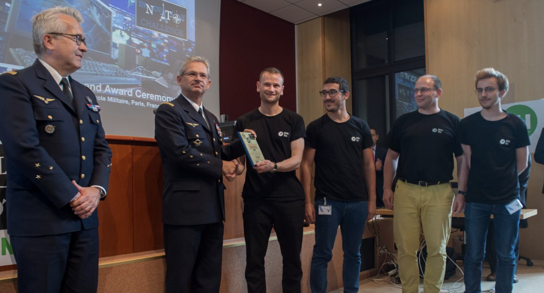
Figure 14: General Maurice, Supreme Commander Mercier, and our team
Thanks to Hicham El Boukkouri & Léo Dreyfus-Schmidt for their review of this blog post.
Note that this post was at first published on Dataiku’s technical blog on Medium.
Update: Our model has been improved recently by Stuparu et al. 2020 and published in Sensors!